Below is a review I wrote for a CUP journal (The Mathematical Gazette) about a recently published text on mathematics in ancient Egypt
Mathematics in ancient Egypt, a contextual history by Annette Imhausen, pp 234, £21.05 (hard), ISBN 978-0-691-11713-3, Princeton University Press (2016)
This is an excellent book that falls mid-way between a specialised and general readership.
Abstractions made possible through mathematics, developed by the ancient Egyptian scribes, placed them in the seats of power.
The starting point for this book is the early prehistory and dynastic developments of number notation in both hieroglyphic and hieratic script (i.e. ‘printed and handwritten’ script). The basis of number systems in Egypt was 10, however, it was without place values and therefore with numerous hieroglyphic signs such as a coiled rope for 100 (the author suggests this may be derived from a measuring rope of 100 standard cubits used to establish field lengths for tax purposes). The earliest use of these numbers on ‘tags’ to record quantities of textiles with others on stela recording tributes. The book is richly illustrated throughout by clear line drawings and photographs of artefacts.
Developments in mathematics during the Old Kingdom, a time of political stability and (consequent) prosperity, occurred but sadly surviving written evidence is scarce. The author illustrates developments through secondary references such as the success of scribes in managing revenues and completing other administrative tasks. The author argues that the establishment of a lunar calendar at this time adds evidence to the scribes understanding of mathematics, not least due to the complexities of marrying observed solar and lunar cycles. The author also reports hints of the later developments in the analysis of gradients from findings at Saqqara.
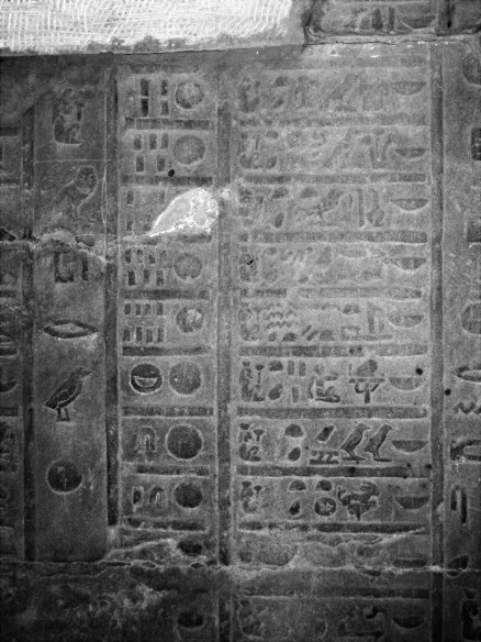 Calendar from Kom Ombo (my photograph from Egypt)
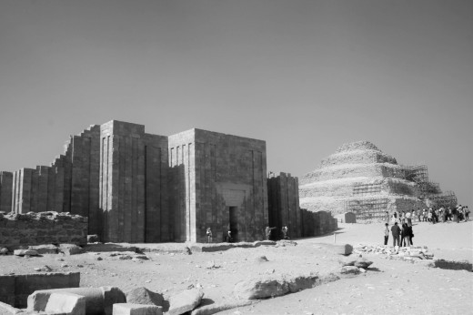 Saqqara (my photograph from Egypt)
In the Middle Kingdom (2055-1650 BCE), following on from an intermediate period when climatic change led to famine, the breaking down of the central administration where scribes had developed and established their mathematics, the first mathematical texts are extant and appear to be derived from an educational context. They teach mathematics a scribe would need in daily work: calculating volumes of granaries, rations, ratios and solving, as the author calls them, ‘bread and beer problems’.
The extant mathematical texts from this period, as one would expect from such a scholarly work, are carefully selected to illustrate developments, and their mathematics clearly explained. Gems from this period include calculating the volume of a truncated pyramid, methods of arithmetic, fractions and in particular the 2/n tables that were crucial to the scribe’s calculations. It is in the use of these methods indicated in non-mathematical texts and tomb models that give an insight into the mathematics that existed; the author richly paints a picture of life in Egypt through examples of its use in calculating rations, and photographs of models from tombs with lines of scribes busying away writing alongside grain stores.
It is not surprising with the magnificent scale of architectural remains visible today, that much of the extant mathematical texts reveal efficient and detailed methods for scribes to use in metrology. The author explains sample methods from texts for calculations of area: perhaps of particular note are the methods for calculation of circular land areas based only on diameters (showing no knowledge of pi), and triangle area calculations that evidence no understanding of what we now call as the ‘rule of Pythagoras’. Contrast this with calculations in near contemporaneous China that clearly indicate both approximation to pi, and ‘Pythagoras’, were well known.
In the New Kingdom (1550-1069 BCE), the dynasties best-known today, the author notes it is surprising that more mathematics texts are not extant. During this period mathematical education remained at the heart of a trainee scribe’s studies. Along with the few scraps of mathematical texts the author points to tombs with the depictions of scribes with measuring ropes surveying in the fields.
One of the joys of translating early mathematical texts is the picture they paint of daily life. The author, through the use of mathematics for administrative purposes, reveals the richness of the lives of the elite with references to calculations involving precious stones, woods, ivories, fruits etc. Other essential, at the time, methods for constructing brick ramps and the transport of Obelisks were also known and carefully detailed in the book.
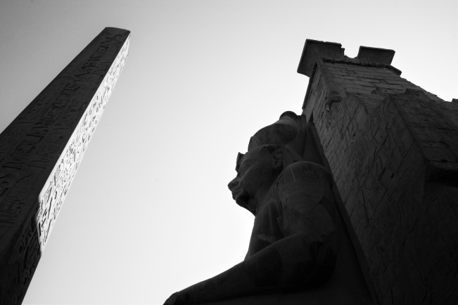
Luxor (my photograph from Egypt)
From this period there are many fragmentary texts that refer to mathematical education and one letter in particular selected by the author will have resonance for the readers of The Gazette: from (presumably) a parent to a student scribe it admonishes him to work hard saying ‘He who works in writing (mathematics) is not taxed, he has no dues (to pay)’.
Not surprisingly, due to the wealth of funerary objects that remain, the author details in them the evidence for use of mathematics, and for numerology in spells contained in the Book of the Dead.
The author deftly deals with speculations that abound by fanciful writers who are keen to project back in time the use of mathematical methods known today: theories that have been taken as ‘truth’ which do not stand up to rigorous studies of the evidence. However, the author does briefly speculate, rather convincingly, about Egyptian conceptualisation of space referencing well illustrated tomb carvings and geometrical problems.
The final chapter of the book details the Greco-Roman periods, a time the author concludes when more mathematical knowledge was transferred from Egypt to Greece than vice versa: that is one suggestion readers of The Gazette might use in conversations with colleagues in their Classics departments.
This was a time rich in extant mathematical texts that enable comparison with earlier methods of arithmetic. As in many other early mathematical texts they are presented as problems with worked solutions, several illuminating examples are included in this book. I was pleased to see the author refrained from trying to assign paths of transmission to specific mathematical knowledge as this is notoriously difficult and often vacuous: details the distinctive ‘pole against wall’ problems re surfaced at this time and their algorithmic solutions are carefully explained.
This book richly demonstrates how mathematics played a central role in ancient Egyptian culture. It clearly distinguishes the Egyptian mathematics from developments in Mesopotamia (where the sexagesimal number system was used) and places it as a distinct and valuable contribution to the development of mathematical knowledge. The result of ten years of research, this keenly priced book stands head and shoulders above others that purport to report on mathematics in ancient Egypt.


 (with the induced topology) as discussed in the previous two posts.
 in the variables
  and
and  defines a plane curve affine variety
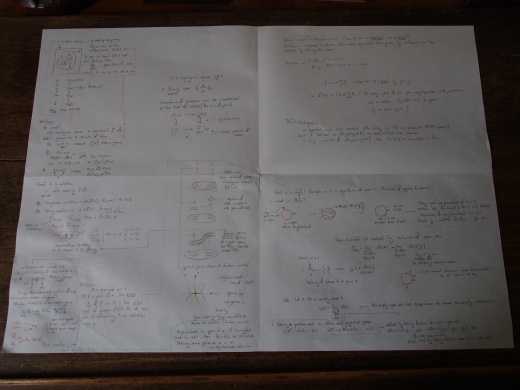
  . Below is the variety for the plane elliptic curve
  .
.
 in
in  is an affine variety. It is the intersection of an ellipse
  and a hyperbola
  .
.
 . In
. In  these are; spheres, ellipsoids, paraboloids, and hyperboloids in
  .
. and an elliptic paraboloid
 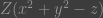 .
.

 and a hyperboliod of two sheets
  .
.

 and
and  that is a `figure of eight’ curve in
 in
in  and the surface
  in
in  are irreducible hyper-surfaces. These are visualised below; the first has components that are connected in Euclidean topology, the second has five components that meet at four singular points.

 , is defined as
 .
. , integer mutilples of
  , is
, is  . The radical ideal of
  is
is  is an algebraically closed field with
 ![A=k[x_1,\dots ,x_n]](https://s0.wp.com/latex.php?latex=A%3Dk%5Bx_1%2C%5Cdots+%2Cx_n%5D&bg=3c3c3c&fg=999999&s=0&c=20201002) and
and  a polynomial that vanishes at all points of
  , then
  for some integer
  .
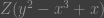
. are subsets of
  , then
  .
. are subsets of
  .
. ,
,  of
of  .
. ,
,  . This is a consequence of Definition 2.2.
 ,
,  , the closure of
  .
. of a commutative ring
  is prime if it has the following properties:
 such that
  , then
  or
or  ,
, , the maximal ideals are the principle ideals generated by a prime number.
 correspondence
 ![\{points\; in \; {A_k}^n\}\Leftrightarrow \{ maximal \; ideals \; of \; k[x_1, \dots, x_n]\}](https://s0.wp.com/latex.php?latex=%5C%7Bpoints%5C%3B+in+%5C%3B+%7BA_k%7D%5En%5C%7D%5CLeftrightarrow+%5C%7B+maximal+%5C%3B+ideals+%5C%3B+of+%5C%3B+k%5Bx_1%2C+%5Cdots%2C+x_n%5D%5C%7D&bg=3c3c3c&fg=999999&s=0&c=20201002) .
.![k[x_1,\dots ,x_n]](https://s0.wp.com/latex.php?latex=k%5Bx_1%2C%5Cdots+%2Cx_n%5D&bg=3c3c3c&fg=999999&s=0&c=20201002) has a zero in
has a zero in  be a finite algebraic set.
  is generated by the function
  , and
, and  so
so  is the inverse of
  .
. is an affine variety iff its ideal
 ![I(X)=k[x_1, \dots, x_n]](https://s0.wp.com/latex.php?latex=I%28X%29%3Dk%5Bx_1%2C+%5Cdots%2C+x_n%5D&bg=3c3c3c&fg=999999&s=0&c=20201002) is a prime ideal.
is a prime ideal. has a dimension of
  as single points are the only irreducible closed subsets of
  is an irreducible polynomial in
 ![A=k[x_1, \dots , x_n]](https://s0.wp.com/latex.php?latex=A%3Dk%5Bx_1%2C+%5Cdots+%2C+x_n%5D&bg=3c3c3c&fg=999999&s=0&c=20201002) , the affine variety
, the affine variety  is called a surface if
  and a hyper-surface of
  .
. is said to be Noetherian if it satisfies a descending chain condition for closed subsets. For any sequence
  of closed subsets there is an integer
  such that
  . Another way of saying this is that the closed subsets are stationary.
 with a mapping
  . Then
  is inclusion-reversing iff for every pair of sets
  such that
  .
. and
and  .
. maximum ideals in a polynomial ring. (Corollary 2.1)
 that does not have a solution in the real numbers.
 is a set of all
  is called a point and for
  , then
  are called the coordinates of
  .
.![A=k[x_1,\dots,x_n]](https://s0.wp.com/latex.php?latex=A%3Dk%5Bx_1%2C%5Cdots%2Cx_n%5D&bg=3c3c3c&fg=999999&s=0&c=20201002) be the polynomial ring in
be the polynomial ring in  and
and  . If
. If  is a polynomial the set of zeros of f are
  . Generally, if
  is any irreducible subset of
  So an affine algebraic variety is the set of common zeros of a collection of polynomials.
 such that
  . The ideal is generated by
  . e.g the ideals
  of the ring of integers
  . We note that a function
  although the ideals are, of course, different. If
  is and ideal of
  .
. there exists an
  i.e. the ascending chain of ideals terminates.
  . Thus
  can be expressed as the common zero’s of the finite set of polynomials
  such that
  .
. , 3) whenever two or more sets are in
  . A set
  is an open set then its complement (
 is called a closed set. Note we can define a topology on a set
  with subsets
  comprise a topology and
  . Here the point
  and
and  with
with  . Let
. Let ![A=k[x_1]](https://s0.wp.com/latex.php?latex=A%3Dk%5Bx_1%5D&bg=3c3c3c&fg=999999&s=0&c=20201002) be the polynomial ring in one variable over
be the polynomial ring in one variable over 
 and
and  . Every ideal in
  , with all
  . Then
  . Thus the algebraic sets in
  ). The open sets are the empty sets and the complements of the finite subsets.
![k[x_1, \dots, x_n]](https://s0.wp.com/latex.php?latex=k%5Bx_1%2C+%5Cdots%2C+x_n%5D&bg=3c3c3c&fg=999999&s=0&c=20201002) . The operation
. The operation ![k[x_1, \dots ,x_n]](https://s0.wp.com/latex.php?latex=k%5Bx_1%2C+%5Cdots+%2Cx_n%5D&bg=3c3c3c&fg=999999&s=0&c=20201002) or an ideal to an algebraic set. With the following definition we establish a two way correspondence.
or an ideal to an algebraic set. With the following definition we establish a two way correspondence. we call the ideal
 ![I(X):=\lbrace f \in k[x_1, \dots, x_n] ; f(P)=0 \; for \; all \; P \in X \rbrace \subset k[x_1,\dots, x_n]](https://s0.wp.com/latex.php?latex=I%28X%29%3A%3D%5Clbrace+f+%5Cin+k%5Bx_1%2C+%5Cdots%2C+x_n%5D+%3B+f%28P%29%3D0+%5C%3B+for+%5C%3B+all+%5C%3B+P+%5Cin+X+%5Crbrace+%5Csubset+k%5Bx_1%2C%5Cdots%2C+x_n%5D+&bg=3c3c3c&fg=999999&s=0&c=20201002) Hence we have defined the following two way correspondence; we have an operation
Hence we have defined the following two way correspondence; we have an operation 
 . If
. If  , if
, if  , otherwise there are two values for
  .
. around the complex origin, the square root of this
  which gives opposite values at
  and
and  . If in
  we travel a path around any of the points
  we move from one of the copies of the complex plain to the other.
![[1,2],\dots,[2n-1,2n]](https://s0.wp.com/latex.php?latex=%5B1%2C2%5D%2C%5Cdots%2C%5B2n-1%2C2n%5D&bg=3c3c3c&fg=999999&s=0&c=20201002) of
of  meet: this results in a compact surface with
  handles. Such objects are called surfaces of genus
  , which results in a surface of genus

